Stable Distributions
3. Other features
[this page | pdf | references | back links]
Return
to Abstract and Contents
Next
page
3.1 Three special cases of stable laws, which have
closed form expressions for their probability densities are:
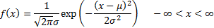
(a) Normal (i.e.
Gaussian).  if
if  has
density
has
density
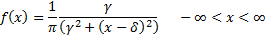
(b) Cauchy.  if has
density
if has
density
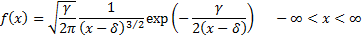
(c) Levy.  if has
density
if has
density
3.2 Generic features of stable distributions noted
by Nolan
(2005) include:
(a) They are unimodal
(b) When  is
small then the skewness parameter is significant, but when is
close to 2 then it matters less and less.
is
small then the skewness parameter is significant, but when is
close to 2 then it matters less and less.
(c) When  (i.e.
the Normal distribution), the distribution has ‘light’ tails and all moments
exist. In all other cases (i.e.
(i.e.
the Normal distribution), the distribution has ‘light’ tails and all moments
exist. In all other cases (i.e.  ), stable distributions
have heavy tails and an asymptotic power law (i.e. Pareto) decay. The term stable
Paretian is thus used to distinguish the
), stable distributions
have heavy tails and an asymptotic power law (i.e. Pareto) decay. The term stable
Paretian is thus used to distinguish the  case
from the Normal case. A consequence of these heavy tails is that not all population
moments exist. If then the population
variance does not exist, and if
case
from the Normal case. A consequence of these heavy tails is that not all population
moments exist. If then the population
variance does not exist, and if  then the population mean
does not exist either. Fractional moments, e.g. the
then the population mean
does not exist either. Fractional moments, e.g. the  ’th
absolute moment, defined as
’th
absolute moment, defined as  ,
exist if and only if
,
exist if and only if  (if ). Of
course all sample moments exist, if there are sufficient observations in
the sample, but these may exhibit unstable behaviour as the sample size
increases if the corresponding population moment does not exist.
(if ). Of
course all sample moments exist, if there are sufficient observations in
the sample, but these may exhibit unstable behaviour as the sample size
increases if the corresponding population moment does not exist.
3.3 Linear combinations of independent stable
distributions with the same index, , are stable. If 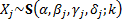 for
for  then
then
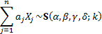
where:

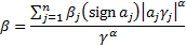
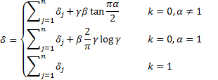
In this generalisation of the definition of stable
distributions given in Section 1.3 it is
essential for the ’s to be the same. Adding
stable random variables with different ’s
does not result in a stable law.
NAVIGATION LINKS
Contents | Prev | Next