Performance Measurement Theory
2. Mathematics of multi-period analysis
[this page | pdf | references | back links]
Return to
Abstract and Contents
Next page
2.1 Suppose that we are interested in calculating
the rate of return on a portfolio from time 0 to time 1 using some suitable
units of time. Suppose that there are n new money payments into or out
of the portfolio in the period of value  (positive for
inflows, negative for outflows) occurring at times
(positive for
inflows, negative for outflows) occurring at times  for
for  .
The are assumed to
be ordered so that
.
The are assumed to
be ordered so that 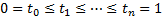 . The market
values at the corresponding points in time (immediately after receipt of the
new money) are
. The market
values at the corresponding points in time (immediately after receipt of the
new money) are  .
Dividend/interest payments are treated as outflows from the relevant stock/bond
sector and inflows into the cash sector, and so net to zero at the total fund
level (unless the income is paid away).
.
Dividend/interest payments are treated as outflows from the relevant stock/bond
sector and inflows into the cash sector, and so net to zero at the total fund
level (unless the income is paid away).
2.2 The time-weighted rate of return for the
period is then 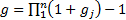 where
where 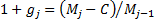 . The
time-weighted rate of return is effectively equivalent to the growth in a unit
net asset value price (were the fund to be unitised and were it to accumulate
income internally, ignoring complications such as bid/offer spreads, etc.) The
positive or negative impact of money arriving or being withdrawn from the
portfolio at opportune or inopportune times is stripped out of the calculation.
Time-weighted rates of return naturally compound up over time, i.e. if the
time-weighted rate of return in one period is
. The
time-weighted rate of return is effectively equivalent to the growth in a unit
net asset value price (were the fund to be unitised and were it to accumulate
income internally, ignoring complications such as bid/offer spreads, etc.) The
positive or negative impact of money arriving or being withdrawn from the
portfolio at opportune or inopportune times is stripped out of the calculation.
Time-weighted rates of return naturally compound up over time, i.e. if the
time-weighted rate of return in one period is  and in the next
is
and in the next
is  then the time
weighted rate of return for the combined period is
then the time
weighted rate of return for the combined period is  where
where
 . This also means
that ‘logged’ returns, i.e.
. This also means
that ‘logged’ returns, i.e.  , naturally add
up through time, i.e.
, naturally add
up through time, i.e.  .
.
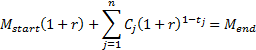
2.3 The money-weighted or internal rate of
return on a fund over the same period, is defined as the ‘sensible’
solution for  to the following
equation (if the are of differing
signs then there will usually be more than one solution, although normally only
one would be intrinsically ‘sensible’):
to the following
equation (if the are of differing
signs then there will usually be more than one solution, although normally only
one would be intrinsically ‘sensible’):
2.4 The time-weighted rate of return and the
money-weighted rate of return are thus the same if there have been no cash
flows during the period.
2.5 One nearly always assumes that  . The internal
rate of return can therefore be approximated by the formula
. The internal
rate of return can therefore be approximated by the formula  , where the contribution
to return (
, where the contribution
to return ( ), net new
money (
), net new
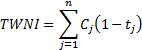
money ( ), time-weighted
net investment (
), time-weighted
net investment ( ), and mean
fund (
), and mean
fund ( ), are defined as
follows:
), are defined as
follows:


2.6 The internal rate of return is the (constant)
interest rate that a bank account would need to provide (possibly negative) to
return the same amount at the end of the period as the portfolio, given the
same new money flows and the same start market value. It is therefore the same
as the money-weighted rate of return and so again does not naturally compound
up over time.
2.7 Calculating the time-weighted rate of return in
principle involves valuations whenever there is a cash flow. This can be time
consuming, unless you have an exceptionally good valuation engine (and even
then is potentially impossible if you wish to value at the exact intra-day
point of time at which a particular trade takes place).
2.8 In practice, therefore, performance measurers
often merely chain-link internal rates of return. This is because the money
weighted and time weighted rates of return are the same if there are no
intra-period new money flows. So, if you calculate internal rates of return
sufficiently often and chain-link them together then the result will always
tend to the time-weighted rate of return.
In certain other special circumstances, the money-weighted
and time-weighted rates of return are also identical. Normally, cash flows and
market values will be expressed in some base currency, but suppose we
generalise the calculation of money-weighted rates of return so that it can
include an arbitrary calculation numeraire, which is worth  in the base
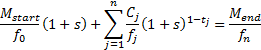
currency at time The money-weighted
rate of return then becomes where
in the base
currency at time The money-weighted
rate of return then becomes where 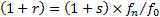 and where
  is
the solution to:
is
the solution to:
2.9 The money-weighted rate of return described
above is then merely a special case of this calculation with a constant (in
base currency) numeraire. Suppose that we choose  , where
  corresponds to
the true cumulative time-weighted return from time 0 to time Then
corresponds to
the true cumulative time-weighted return from time 0 to time Then  and
the money-weighted rate of return, , will (in this
numeraire) be identical to the time-weighted rate of return .
If closely
approximates to
and
the money-weighted rate of return, , will (in this
numeraire) be identical to the time-weighted rate of return .
If closely
approximates to  then will
closely approximate to 0, and the approximation
then will
closely approximate to 0, and the approximation 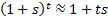 will be very
good. The money-weighted rate of return using such a numeraire will then be
very similar to the true time-weighted rate of return. If the new money flows
are small in relation to start and end market values then the
money-weighted rate of return will also be very similar to the true
time-weighted rate of return, irrespective of the calculation numeraire.
will be very
good. The money-weighted rate of return using such a numeraire will then be
very similar to the true time-weighted rate of return. If the new money flows
are small in relation to start and end market values then the
money-weighted rate of return will also be very similar to the true
time-weighted rate of return, irrespective of the calculation numeraire.
2.10 The calculation numeraire can be differentiated
from the presentation numeraire used to express the results of the
calculation, which will normally be the base currency of the portfolio. If the
presentation numeraire is  then the rates
of return would be restated to be
then the rates
of return would be restated to be  where
where 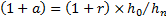 .
.
2.11 The above approach requires not only fund
holding and valuation price data but also information on the prices at which
individual transactions were carried out. If these are difficult to obtain then
an alternative, less exact, methodology involves buy and hold
attribution. In this methodology, the return on each line of stock is imputed
merely from market data over a given period (usually daily) on the assumption
that no transactions have taken place. Such an approach produces the same
answer as a true transactions-based analysis either if no transactions occur or
if they occur at the prices assumed in the algorithm. Unfortunately this
approximation can lead to significant residuals for funds with high turnover or
subject to significant dealing costs.
NAVIGATION LINKS
Contents | Prev | Next