Calculation of weighted moments and
cumulants of probability distributions and samples
[this page | pdf | references]
Equally-weighted statistics
The aggregate characteristics of probability distributions
and data samples are commonly analysed using a small number of statistics
corresponding to their first few moments, namely:
(a) The mean of the
distribution/sample,  , see MnMean, where:

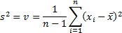
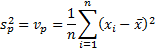
(b) The ‘sample’ and the
‘population’ variance,  and
and  respectively and
the corresponding ‘sample’ and ‘population’ standard deviation,
respectively and
the corresponding ‘sample’ and ‘population’ standard deviation,  and
and
 of the
distribution/sample, see MnVariance,
MnPopulationVariance,
MnStdev and MnPopulationStdev,
where:
of the
distribution/sample, see MnVariance,
MnPopulationVariance,
MnStdev and MnPopulationStdev,
where:
In mathematical texts, is often referred
to as  and as
  .
.
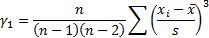
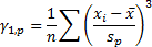
(c) The skew (i.e.
‘skewness’) of the distribution/sample,  , see MnSkew, where:
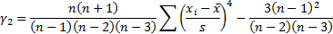
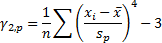
(d) The kurtosis (or more
precisely the ‘excess’ kurtosis),  , of the
distribution/sample, see MnKurt,
where:
, of the
distribution/sample, see MnKurt,
where:
We see that the ‘sample’ variance differs from the
‘population’ variance by a factor of  representing the
loss of one degree of freedom when calculating the mean. This adjustment is
needed to ensure that the sample variance is an unbiased estimate of the
underlying population variance if the distribution is Normal, for finite sized
samples. In the large sample limit, i.e. where
representing the
loss of one degree of freedom when calculating the mean. This adjustment is
needed to ensure that the sample variance is an unbiased estimate of the
underlying population variance if the distribution is Normal, for finite sized
samples. In the large sample limit, i.e. where  ,
the two become equal.
,
the two become equal.
The formula for the skew and kurtosis given above are
properly ‘sample’ rather than ‘population’ measures. Both are dimensionless
quantities, and thus invariant to changes in the ‘scale’ of the distribution
(and its ‘location’) (i.e. if every element of the sample  was replaced by
  , where
  (the
(the
 representing a
change of scale, and the
representing a
change of scale, and the  representing a
change in location) then the skew and kurtosis would remain unaltered. We could
if we wished also define ‘population’ equivalents, see MnPopulationSkew, and
MnPopulationKurt,
where:
representing a
change in location) then the skew and kurtosis would remain unaltered. We could
if we wished also define ‘population’ equivalents, see MnPopulationSkew, and
MnPopulationKurt,
where:
Not equally-weighted
statistics
In some circumstances different elements of a sample should
be given different weights in the formulation of views regarding the overall
probability distribution. For example, there may be greater errors known to be
associated with some specific values used in constructing the sample, so less
credibility should be attached to them when deciding on the overall shape of
the distribution.
Given different weights,  to attach to each
data point (which might, for example, be associated with the square of the
standard error being ascribed to the relevant data point, say
to attach to each
data point (which might, for example, be associated with the square of the
standard error being ascribed to the relevant data point, say  ), derivation of
corresponding weighted ‘population’ statistics is relatively simple, e.g. the
weighted mean,
), derivation of
corresponding weighted ‘population’ statistics is relatively simple, e.g. the
weighted mean,  , the weighted
population variance,
, the weighted
population variance,  , the weighted
population standard deviation
, the weighted
population standard deviation  , the weighted
population skew,
, the weighted
population skew,  , and the weighted
population kurtosis,
, and the weighted
population kurtosis,  , see MnWeightedMean, MnWeightedPopulationVariance,
MnWeightedPopulationStdev,
MnWeightedPopulationSkew
and MnWeightedPopulationKurt,
may be defined as follows (dropping the explicit indexing of the summation
element to simplify the formulae):
, see MnWeightedMean, MnWeightedPopulationVariance,
MnWeightedPopulationStdev,
MnWeightedPopulationSkew
and MnWeightedPopulationKurt,
may be defined as follows (dropping the explicit indexing of the summation
element to simplify the formulae):

More difficult is to identify the correct way to incorporate
an appropriate small sample size adjustment to incorporate the right number of
degrees of freedom. Different commentators (or at least software providers
providing software downloadable from the Internet) appear to use different
approaches, particularly when deriving a suitable measure of weighted ‘sample’
skew.
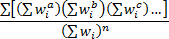
The Nematrian website adopts the approach that small sample
size adjustment factors, at least for the simpler moments/cumulants, should
involve scale invariant factors that are reciprocals of expressions taking the
following form (for suitable combinations of  where
where
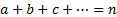 ,
,  being
the ‘order’ of the relevant measure) which reproduce the equally-weighted
adjustment factors for cases where
being
the ‘order’ of the relevant measure) which reproduce the equally-weighted
adjustment factors for cases where  for
for  and
and
 for
for  :
:
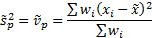
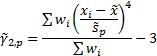
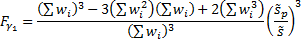
This implies that the most appropriate definitions of the weighted
sample variance,  , the weighted
sample standard deviation
, the weighted
sample standard deviation  and the weighted
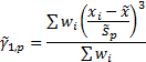
sample skew,
and the weighted
sample skew,  , see MnWeightedVariance,
MnWeightedStdev and
MnWeightedSkew, are:
, see MnWeightedVariance,
MnWeightedStdev and
MnWeightedSkew, are:


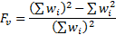
where
Using this methodology it is less clear exactly what small
sample size adjustment we should make when calculating a weighted (sample)
kurtosis measure, but see Rimoldini
(2013). In any case, some commentators such as Press et al.
(2007) suggest that kurtosis (and skew) “should be used with caution, or
better yet, not at all”. Kemp (2009)
also questions the appropriateness of using skew and kurtosis to identify how
non-Normal is a distributional form, see also TVaRForCubicQuantileQuantileRelationships.
The corresponding Cornish-Fisher
approximation that might otherwise be used to extrapolate the shape of the
distributional form seems in general to give inappropriate weight to the wrong
parts of the distributional form when assessing the extent of non-Normality.
Some software systems also allow users to calculate sample
‘moments’ relative to a predefined value, rather than the sample mean, but this
is not currently possible using existing pre-defined Nematrian web service
functions. It is not obvious to us whether it would be particularly useful in
practice. For example, Press et
al. (2007) note that using the formula defined above for the
(equally-weighted) sample skew has a standard error, if the sample is drawn
from a Normal distribution, of approximately  . However, if we replace
the in its definition
by the true mean of the distribution then its standard error rises to
approximately
. However, if we replace
the in its definition
by the true mean of the distribution then its standard error rises to
approximately  . The corresponding
approximate standard errors for kurtosis are
. The corresponding
approximate standard errors for kurtosis are  and
and  respectively. Thus
the computation of both skew and kurtosis becomes less accurate if we
use the true mean in their formulae! For ease of reference, the and formulae are
available directly using MnConfidenceLevelSkewApproxIfNormal
and MnConfidenceLevelKurtApproxIfNormal.
respectively. Thus
the computation of both skew and kurtosis becomes less accurate if we
use the true mean in their formulae! For ease of reference, the and formulae are
available directly using MnConfidenceLevelSkewApproxIfNormal
and MnConfidenceLevelKurtApproxIfNormal.
Weighted correlation correficients, weighted covariances and
weighted population covariances are defined in an equivalent manner, see MnWeightedCorrelations,
MnWeightedCovariances
and MnWeightedPopulationCovariances
respectively.