Quantitative Return Forecasting
2. Traditional time series analysis
[this page | pdf | references | back links]
Return to Abstract and
Contents
Next page
2.1 Consider first a situation where we only have
one time series where we are attempting to forecast future values from observed
past values. For example, the time series followed by a given variable might be
governed by the following relationship, where the value at time t of the
variable is denoted by 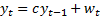 where
where
 is
constant.
is
constant.
2.2 This is a linear first order difference
equation. A difference equation is an expression relating a variable
 to
its previous values. The above equation is first order because only the
first lag (
to
its previous values. The above equation is first order because only the
first lag ( )
appears on the right hand side of the equation. It is linear because it
expresses as
a linear function of and
the innovations
)
appears on the right hand side of the equation. It is linear because it
expresses as
a linear function of and
the innovations  .
are
often treated as random variables, but we do not always need to do this.
.
are
often treated as random variables, but we do not always need to do this.
2.3 Such a model of the world is also an autoregressive
model, with a unit time lag and is therefore typically referred to as an  model.
It is also time stationary, since is constant. Nearly all
linear time series analysis assumes time invariance. We could however introduce
secular changes by assuming one of the variables on which the time series is
based is a dummy variable linked to time. An example commonly referred to in
the quantitative investment literature is a dummy variable set equal to 1 in
January but 0 otherwise, to identify whether there is any ‘January’ effect.
model.
It is also time stationary, since is constant. Nearly all
linear time series analysis assumes time invariance. We could however introduce
secular changes by assuming one of the variables on which the time series is
based is a dummy variable linked to time. An example commonly referred to in
the quantitative investment literature is a dummy variable set equal to 1 in
January but 0 otherwise, to identify whether there is any ‘January’ effect.
2.4 If we know the value  at
at
 then we find using recursive
substitution that
then we find using recursive
substitution that 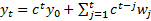 .
We can also determine the effect of each individual
on, say,
.
We can also determine the effect of each individual
on, say,  ,
the value of
,
the value of  that is
  time
periods further into the future value than .
This is sometimes called the dynamic multiplier
time
periods further into the future value than .
This is sometimes called the dynamic multiplier  .
If
.
If  then
such a system is stable, in the sense that the consequences of a given
change in will
eventually die out. It is unstable if
then
such a system is stable, in the sense that the consequences of a given
change in will
eventually die out. It is unstable if  .
An interesting possibility is the borderline case where
.
An interesting possibility is the borderline case where  , when
the output variable is
the sum of its initial starting value and historical inputs.
, when
the output variable is
the sum of its initial starting value and historical inputs.
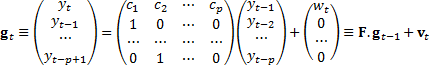
2.5 We can generalise the above dynamic system to
be a linear p’th order difference equation by making it depend on the
first  lags along with the current
value of the innovation (input value) ,
i.e.
lags along with the current
value of the innovation (input value) ,
i.e.  .
This can be rewritten in vector/matrix form as a first order difference
equation, but relating to a vector, if we define the vector as follows:
.
This can be rewritten in vector/matrix form as a first order difference
equation, but relating to a vector, if we define the vector as follows:
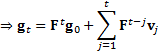
2.6 These sorts of dynamic systems have richer
structures than simple scalar difference equations. For a p’th order
equation we have:  (if
(if
 is
the element in the i’th row and k’th column of
is
the element in the i’th row and k’th column of  ).
To analyse the characteristics of such a system in more detail, we first need
to identify the eigenvalues of
).
To analyse the characteristics of such a system in more detail, we first need
to identify the eigenvalues of  .
These are the values of
.
These are the values of  for which
  where
where
 is
the identity matrix. They are the roots to the following equation:
is
the identity matrix. They are the roots to the following equation:

2.7 A p’th order equation such as this
always has p roots, but some of these may be complex numbers rather than
real ones, even if (as would be the case in practice for investment time
series) all the  are
real numbers. Complex roots correspond to cyclical (sinusoidal) behaviour. We
can therefore have combinations of exponential decay, exponential growth and
sinusoidal (perhaps damped or inflating) behaviour. For such a system to be
stable we require all the eigenvalues to
satisfy
are
real numbers. Complex roots correspond to cyclical (sinusoidal) behaviour. We
can therefore have combinations of exponential decay, exponential growth and
sinusoidal (perhaps damped or inflating) behaviour. For such a system to be
stable we require all the eigenvalues to
satisfy  ,
i.e. for their absolute values all to be less than unity.
,
i.e. for their absolute values all to be less than unity.
2.8 Eigenvalues are closely associated with principal
components analysis. All non-negative definite symmetric  matrices,
 ,
will have
,
will have  non-negative eigenvalues
  and
associated eigenvectors
and
associated eigenvectors  (the
eigenvectors can sometimes be degenerate) that satisfy
(the
eigenvectors can sometimes be degenerate) that satisfy  .
The eigenvalues can be the same in which case the eigenvectors can be
degenerate. The eigenvectors are orthogonal (or can be chosen to be orthogonal
if they are degenerate), so that any n-vector
.
The eigenvalues can be the same in which case the eigenvectors can be
degenerate. The eigenvectors are orthogonal (or can be chosen to be orthogonal
if they are degenerate), so that any n-vector  can
be written as
can
be written as  .
.
2.9 The principal components are the eigenvectors
of the relevant covariance matrix corresponding to the largest eigenvalues,
since they explain the greatest amount of variance when averaged over all
possible positions. This is because .
There is no fundamental reason why all stocks should be given equal weight in
this averaging process. Different weighting schemas result in different vectors
being deemed ‘principal’.
NAVIGATION LINKS
Contents | Prev | Next