Enterprise Risk Management Formula Book
4. Statistical distributions
[this page | pdf | back links]
4.1 Probability distribution terminology
Suppose a (continuous) real valued random variable,  , has a probability density function
(or pdf)
, has a probability density function
(or pdf)  . Then
the probability of taking
a value between
. Then
the probability of taking
a value between  and
and  where
where  is
infinitesimal,
is
infinitesimal, 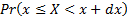 , is
, is  .
.
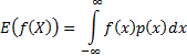
The expected value of a function  (given
this pdf) is defined (if the integral exists) as follows and is also sometimes
written
(given
this pdf) is defined (if the integral exists) as follows and is also sometimes
written  :
:
For to be a
pdf it must exhibit certain basic regularity conditions including  .
.
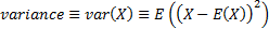
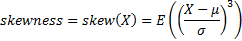
The mean,
variance, standard deviation, cumulative distribution
function (cdf or just distribution function), inverse cumulative
distribution function (inverse cdf or just inverse function
or quantile function), skewness (or skew),
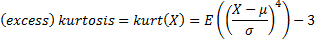
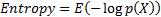
(excess) kurtosis, mean
excess function,  ’th central
and non-central moments and entropy are defined as:
’th central
and non-central moments and entropy are defined as:


The cumulants (sometimes called semi-invariants),
 , of a
distribution, if they exist, are defined via the cumulant generating function,
i.e. the power series expansion
, of a
distribution, if they exist, are defined via the cumulant generating function,
i.e. the power series expansion  of
of  . The
mean, standard deviation, skewness and (excess) kurtosis of a distribution are
. The
mean, standard deviation, skewness and (excess) kurtosis of a distribution are  ,
,  ,
, 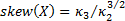 and
and 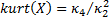
The mode
of a (continuous) distribution, i.e.  , is the
value at which is
largest.
, is the
value at which is
largest.
The median,
upper quartile and lower quartile etc. (or more generally percentile) of a
(continuous) distribution are  ,
,  ,
,  etc. (or
 ) respectively.
Definitions of the above for discrete real-valued random
variables are similar as long as the integrals involved are replaced with sums
and the probability density function by the probability mass function
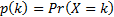 , i.e.
the probability of taking
the value
, i.e.
the probability of taking
the value  .
.
Some of the above are not well defined or are infinite for
some probability distributions.
If a discrete random variable can only take values which are
non-negative integers, i.e. from the set  then
the probability generating function is defined as:
then
the probability generating function is defined as:

Characteristic functions and (if they exist) central moments
and moment generating functions can nearly always be derived from non-central
moments by applying the binomial expansion, e.g.  ,
,  etc.
(where is a
constant)
etc.
(where is a
constant)
The domain (more fully, the domain of definition
or range) of a (continuous) probability distribution is the set of
values for which the probability density function is defined. The support
of a (discrete) probability distribution is the set of values of for
which  is
non-zero. The usual convention for a continuous function is to define the
distribution only where the probability density function would be non-zero and
for a discrete function (usually) to define the distribution only where the
probability mass function is non-zero, in which case the domain/range and
support coincide.
is
non-zero. The usual convention for a continuous function is to define the
distribution only where the probability density function would be non-zero and
for a discrete function (usually) to define the distribution only where the
probability mass function is non-zero, in which case the domain/range and
support coincide.
The survival function (or reliability function)
is the probability that the variable takes a value greater than (i.e.
probability a unit survives beyond time if is
measuring time) so is:

The hazard function
(also known as the failure rate) is the ratio of the pdf to the survival
function, so is:
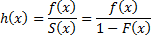
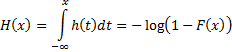
The cumulative hazard function is the integral of the
hazard function (i.e. the probability of failure at time given
survival to time , if is
measuring time) so is:
Definitions, characteristics and common interpretations of a
variety of (discrete and continuous) probability distributions are given in
Appendix A.
The probability that  occurs
given that occurs,
occurs
given that occurs,
 is
defined for
is
defined for  as:
as:
For discrete random variables, , , the
expected value of  given
that occurs,
given
that occurs,
 is
defined as follows, where
is
defined as follows, where  is the
range of :
is the
range of :

The following relationships apply:

If  is a
vector of (continuous) random variables then its (multivariate) pdf
is a
vector of (continuous) random variables then its (multivariate) pdf  and its
cdf
and its
cdf  satisfy:


The covariance between  and
and  is
is  and the
(Pearson) correlation coefficient is
and the
(Pearson) correlation coefficient is 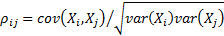 . The
covariance matrix and the (Pearson) correlation matrix for multiple series are
the matrices
. The
covariance matrix and the (Pearson) correlation matrix for multiple series are
the matrices  and
and  which
have as their elements
which
have as their elements  and
and  respectively.
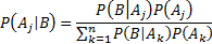
4.2 Bayes theorem
Let  be a
collection of mutually exclusive and exhaustive events with probability of
event
be a
collection of mutually exclusive and exhaustive events with probability of
event  occurring
being
occurring
being  for
for  . Then,
for any event
. Then,
for any event  such
that
such
that  the
probability,
the
probability,  , of occurring
conditional on occurring
(more simply the probability of given )
satisfies:
, of occurring
conditional on occurring
(more simply the probability of given )
satisfies:
A singly conditional probability (i.e. order 1) is
e.g.  . A doubly
conditional probability (i.e. order 2) is e.g.
. A doubly
conditional probability (i.e. order 2) is e.g.  ,
probability of
,
probability of  occurring
given both and
occurring
given both and  take
specific values. Nil-conditioned conditional probabilities (i.e. order
0) are the marginal probabilities, e.g.
take
specific values. Nil-conditioned conditional probabilities (i.e. order
0) are the marginal probabilities, e.g.  . A Bayesian
network (more simply Bayesian net) is a directed acyclical graph where each
node/vertex, say
. A Bayesian
network (more simply Bayesian net) is a directed acyclical graph where each
node/vertex, say  is
associated with a random variable, say (often
a two-valued, i.e. Boolean, random variable) and with a conditional probability
table. For nodes without a parent the table contains just the marginal
probabilities for the values that might
take. For nodes with parents it contains all conditional probabilities for the
values that might
take given that its parents take specified values.
is
associated with a random variable, say (often
a two-valued, i.e. Boolean, random variable) and with a conditional probability
table. For nodes without a parent the table contains just the marginal
probabilities for the values that might
take. For nodes with parents it contains all conditional probabilities for the
values that might
take given that its parents take specified values.
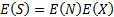
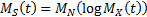
4.3 Compound distributions
If  are
independent identically distributed random variables with moment generating
function
are
independent identically distributed random variables with moment generating
function  and
and  is an
independent non-negative integer-valued random variable then
is an
independent non-negative integer-valued random variable then 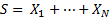 (with
(with  when
when  ) has
the following properties:
) has
the following properties:

For example, the compound Poisson distribution has:  and
and  where
where  and
and 
NAVIGATION LINKS
Contents | Prev | Next