Enterprise Risk Management Formula Book
13. Miscellaneous
[this page | pdf | back links]
13.1 Combining solvency capital requirements using
correlations
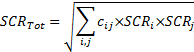
A correlation based combination of individual solvency
capital requirements involves a formula along the lines of:
13.2 Credit risk modelling
A single factor credit portfolio model generally assumes 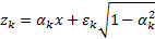 where
where  is
the (standardised) factor return/movement,
is
the (standardised) factor return/movement,  is the exposure of
the
is the exposure of
the  ’th obligor to that
factor and
’th obligor to that
factor and  is the
idiosyncratic noise term for that obligor.
is the
idiosyncratic noise term for that obligor.
If  is the same for
all instruments (e.g. all are assumed to have same correlation with market plus
only an idiosyncratic term) then
is the same for
all instruments (e.g. all are assumed to have same correlation with market plus
only an idiosyncratic term) then 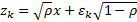 . In such
circumstances and if all obligors have the same probability of default
. In such
circumstances and if all obligors have the same probability of default  say
then probability
say
then probability  that out
of
that out
of  default is:

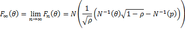
If  is the cumulative
probability that the percentage loss on the portfolio does not exceed
is the cumulative
probability that the percentage loss on the portfolio does not exceed  then
in the well diversified limit (Vasicek’s loss distribution):
then
in the well diversified limit (Vasicek’s loss distribution):
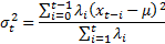
13.3 GARCH models
Risk models may cater for heteroscedasticity by including
GARCH features, e.g. the model might involve formulae along the lines of (in
practice  will slowly evolve
as additional data is received):
will slowly evolve
as additional data is received):


where for, say, a GARCH(1,1) model

RiskMetrics typically uses the following approach for
estimating  (often using
  for some suitably
chosen decay factor
for some suitably
chosen decay factor  ) which can be
viewed as an example of a GARCH approach and/or using weighted moments.
) which can be
viewed as an example of a GARCH approach and/or using weighted moments.
13.4 Linear algebra and principal components
Suppose we have  data series (e.g.
returns) each with
data series (e.g.
returns) each with  observations,
  , that are
coincident in time across the different data series. Suppose the
, that are
coincident in time across the different data series. Suppose the  covariance
matrix of the (empirical) covariances between the different series is
covariance
matrix of the (empirical) covariances between the different series is  . The eigenvalues
and eigenvectors of
. The eigenvalues
and eigenvectors of  are the values of (scalar)
and associated
are the values of (scalar)
and associated  (vector) for which
 . An matrix
has
. An matrix
has  (not necessarily
distinct) eigenvalues and associated eigenvectors. Eigenvectors associated with
distinct eigenvalues are orthogonal, i.e.
(not necessarily
distinct) eigenvalues and associated eigenvectors. Eigenvectors associated with
distinct eigenvalues are orthogonal, i.e.  for
for  .
Orthonormal eigenvectors have
.
Orthonormal eigenvectors have  and for .
For any distinct eigenvalue the associated orthonormal eigenvector is unique up
to a change of sign. If
and for .
For any distinct eigenvalue the associated orthonormal eigenvector is unique up
to a change of sign. If  eigenvalues all
take the same value then it is possible to find
eigenvalues all
take the same value then it is possible to find  orthogonal
eigenvectors corresponding to all of these eigenvalues. For empirical
covariance matrices, is symmetric
non-negative definite (and positive definite if no two data series are
perfectly correlated) and all of its eigenvalues,
orthogonal
eigenvectors corresponding to all of these eigenvalues. For empirical
covariance matrices, is symmetric
non-negative definite (and positive definite if no two data series are
perfectly correlated) and all of its eigenvalues,  , are greater than
or equal to zero. One way of telling if a matrix is positive definite is to
test whether it is possible to apply a Cholesky decomposition to it.
, are greater than
or equal to zero. One way of telling if a matrix is positive definite is to
test whether it is possible to apply a Cholesky decomposition to it.
The eigenvalues and associated eigenvectors of an empirical
covariance matrix may be sorted so that 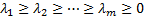 . The first
principal component is the mixture of the underlying (de-meaned) series,
i.e. the
. The first
principal component is the mixture of the underlying (de-meaned) series,
i.e. the 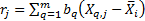 , that corresponds
to the orthonormal eigenvector,
, that corresponds
to the orthonormal eigenvector,  , corresponding to
the largest eigenvalue of . This choice of maximises
, corresponding to
the largest eigenvalue of . This choice of maximises  subject to
  , Other (lesser) principal components
correspond to orthonormal eigenvectors corresponding to smaller eigenvalues.
, Other (lesser) principal components
correspond to orthonormal eigenvectors corresponding to smaller eigenvalues.
13.5 Central limit theorem
Suppose we have a series of independent random variables  each with finite
(bounded) expected value
each with finite
(bounded) expected value  and finite
(bounded) standard deviation
and finite
(bounded) standard deviation  . Suppose
  and
and  are defined as:
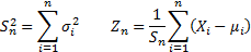
Then subject to certain regularity conditions the
distribution of tends
asymptotically to  (it is exactly if each of the
  is normally
distributed).
is normally
distributed).
13.6 Cornish-Fisher asymptotic expansion
The (4th moment) Cornish-Fisher
asymptotic expansion approximates a standardised QQ-plot via the following
function:

where  and
and  are the skew and
excess kurtosis of the data.
are the skew and
excess kurtosis of the data.
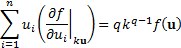
13.7 Euler capital allocation principle
A function  where
where 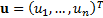 is said to be
homogenous of order if:
is said to be
homogenous of order if:
Suppose we have business lines,
the outcome (loss) to each business line given its current size is  (a random
variable) so the total loss is
(a random
variable) so the total loss is  where for the
current business portfolio the business line allocation is
where for the
current business portfolio the business line allocation is  . Suppose the risk
measure used to determine economic capital is
. Suppose the risk
measure used to determine economic capital is  and that it is
homogeneous of order 1, i.e.
and that it is
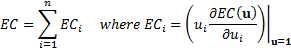
homogeneous of order 1, i.e.  . Then the Euler
capital allocation principle (and, in effect, the Marginal VaR or Internal beta
approach to setting RAROC rates) allocates total economic capital,
. Then the Euler
capital allocation principle (and, in effect, the Marginal VaR or Internal beta
approach to setting RAROC rates) allocates total economic capital,  (technically
a function of the business portfolio allocation,
(technically
a function of the business portfolio allocation,  ) into capital for
each business line,
) into capital for
each business line,  , as follows:
13.8 Equiprobable outcomes for a multivariate normal
distribution
If  where
where  then equiprobable
scenarios (i.e. contours where
then equiprobable
scenarios (i.e. contours where  is constant) are
ellipsoids defined by
is constant) are
ellipsoids defined by  for some constant
value of . The probability
that
for some constant
value of . The probability
that  lies within this
ellipsoid is given by a chi-squared with degrees of
freedom:
lies within this
ellipsoid is given by a chi-squared with degrees of
freedom:

13.9 RAROC, EIC, SHV and SVA
Risk adjusted return on capital (RAROC) is usually defined
as follows, where  = Adjusted
earnings = Earnings – Interest cost – expected loss – funding
cost – other costs and
= Adjusted
earnings = Earnings – Interest cost – expected loss – funding
cost – other costs and  = capital:

Economic income created (EIC) is usually defined as where  =
per unit cost of equity (i.e. hurdle rate):
=
per unit cost of equity (i.e. hurdle rate):

Shareholder value (SHV) and shareholder value added (SVA)
(also known as economic value added, EVA) translate current period return
contribution to overall economic value. Given suitable assumptions about future
growth prospects for a business,  , these are:

NAVIGATION LINKS
Contents | Prev | Next